Independent T-test using SPSS

Independent T-test (simply called t-test unless otherwise stated) helps to compare the mean values between two independent groups. For example,

1. Is there significant difference between the mean income of males and females?
2. Is the difference between mean birthweight of children born to mothers who smoked during pregnancy compared to those who didn't?
3. Does the average systolic blood pressure significantly differ among patients who take drug A and drug B.

From above examples, you might have already guessed that it compares the mean value between two different groups. If we want to compare the means in the same group (e.g. before and after intervention), then we calculate paired-t test.

Criteria for independent sample T-test:

1. Dependent variable should be numeric (ratio scale, e.g. height in cm, weight in kg, income in dollars, etc.)

2. Independent variable should be categorical with 2 categories (e.g. sex with two categories male and female). If the independent variable has more than 2 categories, SPSS allows us to chose 2 categories among them. If we want to compare means among more than 2 categories, we use ANOVA which is extended form of T-test.

Steps of computing Independent-t test using SPSS

Step 1. Open the dataset. I do it on "demo.sav" which is freely available to practice inside your SPSS installation directory.

Step 2: Decide the numeric dependent variable (e.g. income) and independent categorical variable (e.g. gender). Choice of dependent and independent variable depends purely on our research objectives/research hypothesis/research question. 

Step 3: Go to analyze, compare means and independent samples T-test

Step 4: A dialog box appears which asks for test variable and grouping variable. Drag the dependent variable (e.g. income from demo.sav) to test-variable section and independent variable (e.g. gender from demo.sav) to grouping variable section.

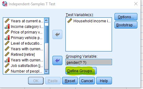
Step 5: Click on define groups and write the symbols/codes in the boxes for two categories of the independent variable which was used during data entry. (In the given sample data demo.sav, m denotes male and f denotes female; you might have your unique code in your dataset) and click on continue.

Step 6: After that you see the following dialog box.

Step 7: When we click on option, we can use our desired confidence interval. By default, it is set as 95%. We can set it to any value we want such as 90% or 99% or 80%. It again depends on our objective. usually, it is set as 95%. So, we may leave it as it is and click continue.

Step 8: Click on ok and you get the output as follows:

Step 9: Interpreting the output: From the given output, you can see that mean income of males was 81.56218 and that of females was 75.73510. Similarly, we can see the t-test value of 0.702 assuming equal variances and the same value assuming unequal variances between male and female groups. The P-values for Levene's test of equality of variance is 0.172 which is greater than 0.05 and so, we can assume equal variance between the groups. Similarly, the P-value is 0.483 (which is seen under the heading sig 2 tailed). We can also see the Confidence interval (CI) for t-test value.

We can conclude from the above table that the mean difference in income among males and females was not statistically significant. (as calculated P-value of 0.483 is less than 0.05 which is the usual assigned level of significance or alpha).

Good luck and see you in the next tutorial!!